Neural Network: Backpropagation nell'Hidden Layer

Calcolo del Gradiente Rispetto ai Pesi

Come già fatto per l’output layer, calcoliamo le derivate parziali della Loss $L$ rispetto a ciascun peso $w^h_{t,s}$ dell’hidden layer.

A differenza di quanto accade per un peso dell’output layer, l’attivazione di un nodo dell’hidden layer può influenzare più nodi dell’output layer. Di conseguenza, per calcolare la derivata rispetto a un parametro dell’hidden layer, dobbiamo sommare i contributi provenienti da tutti i percorsi attraverso i quali quel parametro influenza la Loss. Ad esempio, per calcolare $\partial L/\partial w^h_{1,1}$, dobbiamo considerare sia il percorso che passa attraverso $a^o_1$, sia quello che passa attraverso $a^o_2$. Lo stesso principio vale per gli altri pesi dell’hidden layer:

$$ \require{physics} \begin{align} \pdv{L}{w^h_{1,1}} &= \pdv{L}{a^o_1} \cdot \pdv{a^o_1}{z^o_1} \cdot \pdv{z^o_1}{a^h_1} \cdot \pdv{a^h_1}{z^h_1} \cdot \pdv{z^h_1}{w^h_{1,1}}\\[6pt] &\quad+ \pdv{L}{a^o_2} \cdot \pdv{a^o_2}{z^o_2} \cdot \pdv{z^o_2}{a^h_1} \cdot \pdv{a^h_1}{z^h_1} \cdot \pdv{z^h_1}{w^h_{1,1}}. \end{align} $$

$$ \begin{align} \pdv{L}{w^h_{1,2}} & = \pdv{L}{a^o_1} \cdot \pdv{a^o_1}{z^o_1} \cdot \pdv{z^o_1}{a^h_1} \cdot \pdv{a^h_1}{z^h_1} \cdot \pdv{z^h_1}{w^h_{1,2}}\\[6pt] & + \pdv{L}{a^o_2} \cdot \pdv{a^o_2}{z^o_2} \cdot \pdv{z^o_2}{a^h_1} \cdot \pdv{a^h_1}{z^h_1} \cdot \pdv{z^h_1}{w^h_{1,2}}\\[6pt] \end{align} $$

$$ \begin{align} \pdv{L}{w^h_{2,1}} & = \pdv{L}{a^o_1} \cdot \pdv{a^o_1}{z^o_1} \cdot \pdv{z^o_1}{a^h_2} \cdot \pdv{a^h_2}{z^h_2} \cdot \pdv{z^h_2}{w^h_{2,1}}\\[6pt] & + \pdv{L}{a^o_2} \cdot \pdv{a^o_2}{z^o_2} \cdot \pdv{z^o_2}{a^h_2} \cdot \pdv{a^h_2}{z^h_2} \cdot \pdv{z^h_2}{w^h_{2,1}}\\[6pt] \end{align} $$

$$ \begin{align} \pdv{L}{w^h_{2,2}} & = \pdv{L}{a^o_1} \cdot \pdv{a^o_1}{z^o_1} \cdot \pdv{z^o_1}{a^h_2} \cdot \pdv{a^h_2}{z^h_2} \cdot \pdv{z^h_2}{w^h_{2,2}}\\[6pt] & + \pdv{L}{a^o_2} \cdot \pdv{a^o_2}{z^o_2} \cdot \pdv{z^o_2}{a^h_2} \cdot \pdv{a^h_2}{z^h_2} \cdot \pdv{z^h_2}{w^h_{2,2}}\\[6pt] \end{align} $$

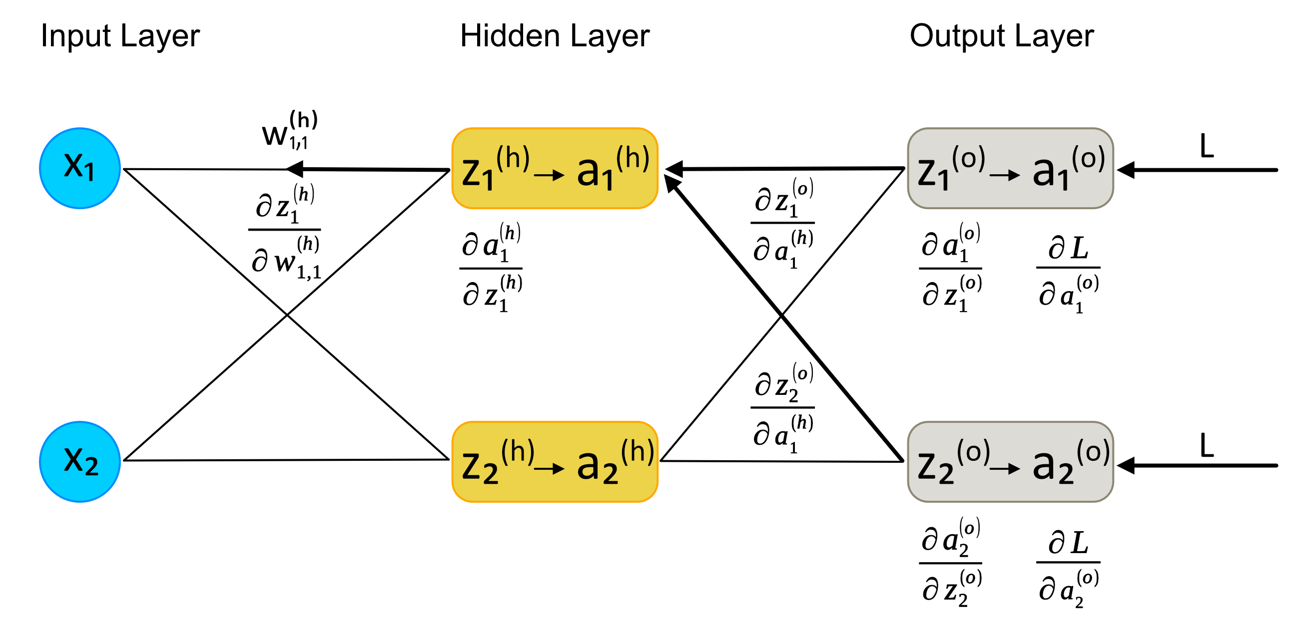
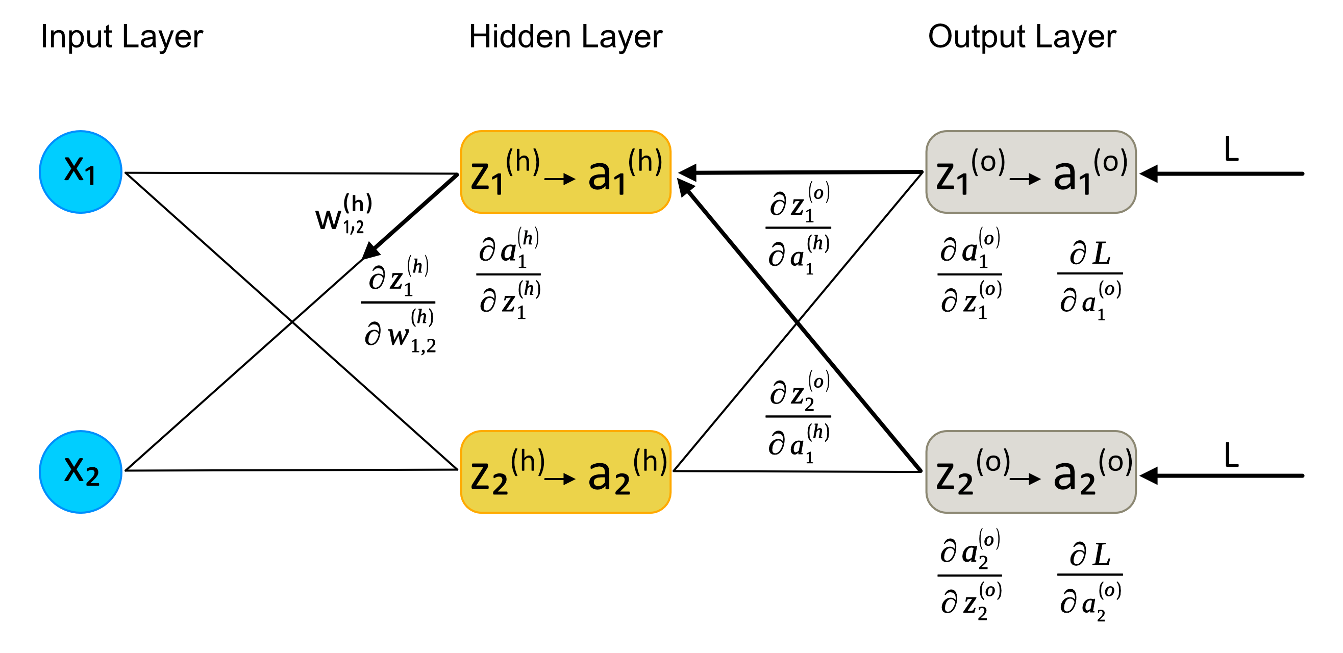
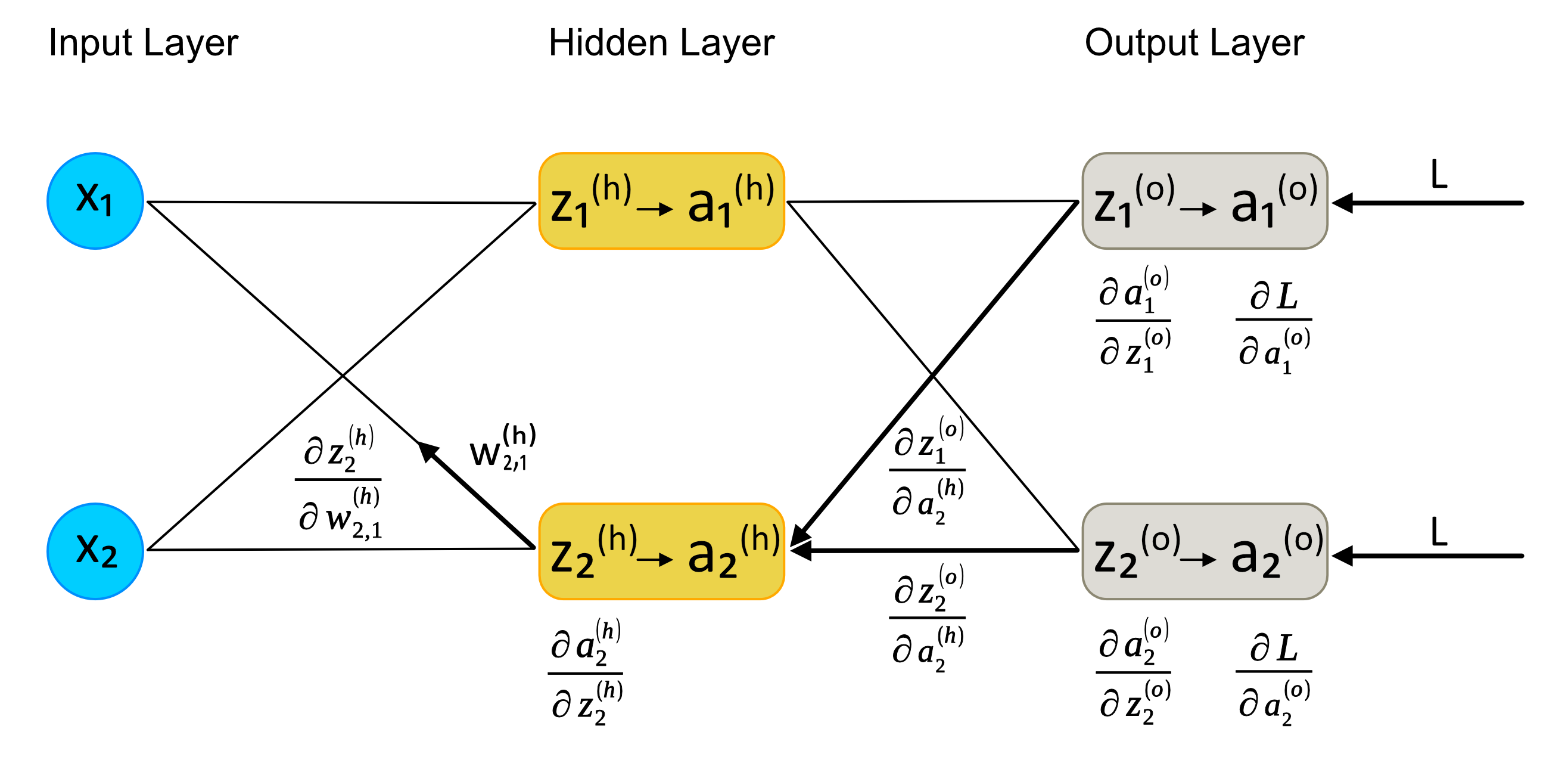
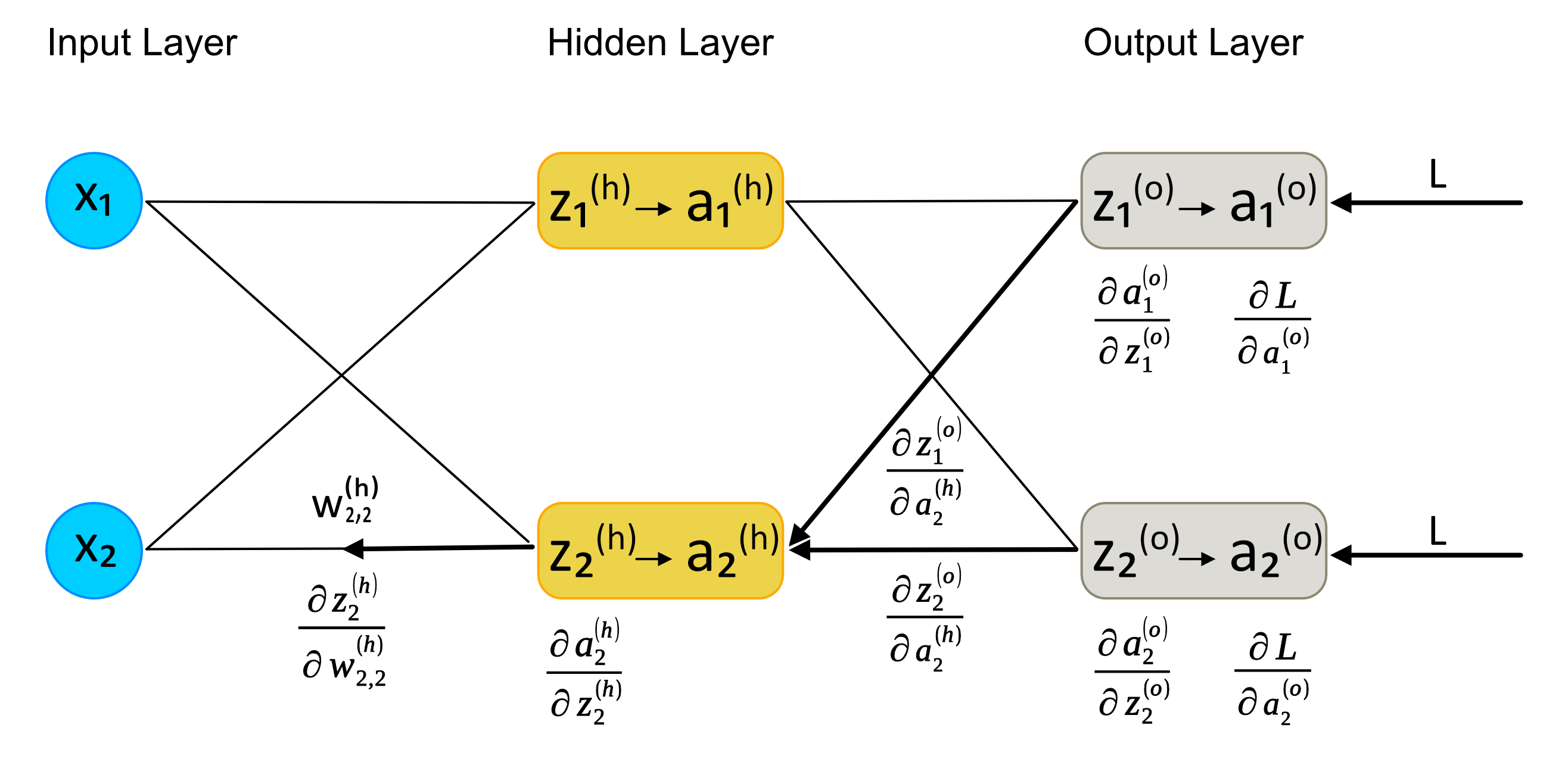
Riassumendo:

$$ \begin{align} \pdv{L}{w^h_{1,1}} & = \pdv{L}{a^o_1} \cdot \pdv{a^o_1}{z^o_1} \cdot \pdv{z^o_1}{a^h_1} \cdot \pdv{a^h_1}{z^h_1} \cdot \pdv{z^h_1}{w^h_{1,1}} + \pdv{L}{a^o_2} \cdot \pdv{a^o_2}{z^o_2} \cdot \pdv{z^o_2}{a^h_1} \cdot \pdv{a^h_1}{z^h_1} \cdot \pdv{z^h_1}{w^h_{1,1}}\\[6pt] \pdv{L}{w^h_{1,2}} & = \pdv{L}{a^o_1} \cdot \pdv{a^o_1}{z^o_1} \cdot \pdv{z^o_1}{a^h_1} \cdot \pdv{a^h_1}{z^h_1} \cdot \pdv{z^h_1}{w^h_{1,2}} + \pdv{L}{a^o_2} \cdot \pdv{a^o_2}{z^o_2} \cdot \pdv{z^o_2}{a^h_1} \cdot \pdv{a^h_1}{z^h_1} \cdot \pdv{z^h_1}{w^h_{1,2}}\\[6pt] \pdv{L}{w^h_{2,1}} & = \pdv{L}{a^o_1} \cdot \pdv{a^o_1}{z^o_1} \cdot \pdv{z^o_1}{a^h_2} \cdot \pdv{a^h_2}{z^h_2} \cdot \pdv{z^h_2}{w^h_{2,1}} + \pdv{L}{a^o_2} \cdot \pdv{a^o_2}{z^o_2} \cdot \pdv{z^o_2}{a^h_2} \cdot \pdv{a^h_2}{z^h_2} \cdot \pdv{z^h_2}{w^h_{2,1}}\\[6pt] \pdv{L}{w^h_{2,2}} & = \pdv{L}{a^o_1} \cdot \pdv{a^o_1}{z^o_1} \cdot \pdv{z^o_1}{a^h_2} \cdot \pdv{a^h_2}{z^h_2} \cdot \pdv{z^h_2}{w^h_{2,2}} + \pdv{L}{a^o_2} \cdot \pdv{a^o_2}{z^o_2} \cdot \pdv{z^o_2}{a^h_2} \cdot \pdv{a^h_2}{z^h_2} \cdot \pdv{z^h_2}{w^h_{2,2}}\\[6pt] \end{align} $$

Possiamo semplificare le espressioni utilizzando i termini $d^o_j$ già introdotti per l’output layer (le derivata parziali di output dei nodi di tale layer):

$$ \begin{align} d^o_1 &= \pdv{L}{z^o_1} = \pdv{L}{a^o_1}\cdot\pdv{a^o_1}{z^o_1}\\[6pt] d^o_2 &= \pdv{L}{z^o_2} = \pdv{L}{a^o_2}\cdot\pdv{a^o_2}{z^o_2} \end{align} $$

Otteniamo quindi:

$$ \begin{align} \pdv{L}{w^h_{1,1}} & = d^o_1 \cdot \pdv{z^o_1}{a^h_1} \cdot \pdv{a^h_1}{z^h_1} \cdot \pdv{z^h_1}{w^h_{1,1}} + d^o_2 \cdot \pdv{z^o_2}{a^h_1} \cdot \pdv{a^h_1}{z^h_1} \cdot \pdv{z^h_1}{w^h_{1,1}}\\[6pt] \pdv{L}{w^h_{1,2}} & = d^o_1 \cdot \pdv{z^o_1}{a^h_1} \cdot \pdv{a^h_1}{z^h_1} \cdot \pdv{z^h_1}{w^h_{1,2}} + d^o_2 \cdot \pdv{z^o_2}{a^h_1} \cdot \pdv{a^h_1}{z^h_1} \cdot \pdv{z^h_1}{w^h_{1,2}}\\[6pt] \pdv{L}{w^h_{2,1}} & = d^o_1 \cdot \pdv{z^o_1}{a^h_2} \cdot \pdv{a^h_2}{z^h_2} \cdot \pdv{z^h_2}{w^h_{2,1}} + d^o_2 \cdot \pdv{z^o_2}{a^h_2} \cdot \pdv{a^h_2}{z^h_2} \cdot \pdv{z^h_2}{w^h_{2,1}}\\[6pt] \pdv{L}{w^h_{2,2}} & = d^o_1 \cdot \pdv{z^o_1}{a^h_2} \cdot \pdv{a^h_2}{z^h_2} \cdot \pdv{z^h_2}{w^h_{2,2}} + d^o_2 \cdot \pdv{z^o_2}{a^h_2} \cdot \pdv{a^h_2}{z^h_2} \cdot \pdv{z^h_2}{w^h_{2,2}}\\[6pt] \end{align} $$

Ricordando che:

$$ \begin{align} z^o_1 &= w^o_{1,1}a^h_1+w^o_{1,2}a^h_2+b^o_1\\[6pt] z^o_2 &= w^o_{2,1}a^h_1+w^o_{2,2}a^h_2+b^o_2 \end{align} $$

abbiamo:

$$ \begin{align} \pdv{z^o_1}{a^h_1} &= w^o_{1,1} & \pdv{z^o_1}{a^h_2} &= w^o_{1,2}\\[6pt] \pdv{z^o_2}{a^h_1} &= w^o_{2,1} & \pdv{z^o_2}{a^h_2} &= w^o_{2,2} \end{align} $$

Per l’hidden layer:

$$ \begin{align} z^h_1 &= w^h_{1,1}x_1+w^h_{1,2}x_2+b^h_1\\[6pt] z^h_2 &= w^h_{2,1}x_1+w^h_{2,2}x_2+b^h_2 \end{align} $$

da cui:

$$ \begin{align} \pdv{z^h_1}{w^h_{1,1}} &= x_1 & \pdv{z^h_1}{w^h_{1,2}} &= x_2\\[6pt] \pdv{z^h_2}{w^h_{2,1}} &= x_1 & \pdv{z^h_2}{w^h_{2,2}} &= x_2 \end{align} $$

Possiamo quindi scrivere:

$$ \begin{align} \pdv{L}{w^h_{1,1}} &= \left( d^o_1w^o_{1,1} + d^o_2w^o_{2,1} \right) \pdv{a^h_1}{z^h_1} \,x_1\\[6pt] \pdv{L}{w^h_{1,2}} &= \left( d^o_1w^o_{1,1} + d^o_2w^o_{2,1} \right) \pdv{a^h_1}{z^h_1} \,x_2\\[6pt] \pdv{L}{w^h_{2,1}} &= \left( d^o_1w^o_{1,2} + d^o_2w^o_{2,2} \right) \pdv{a^h_2}{z^h_2} \,x_1\\[6pt] \pdv{L}{w^h_{2,2}} &= \left( d^o_1w^o_{1,2} + d^o_2w^o_{2,2} \right) \pdv{a^h_2}{z^h_2} \,x_2 \end{align} $$

Definiamo ora:

$$ d^h_j=\pdv{L}{z^h_j} $$

cioè la derivata della Loss rispetto alla combinazione lineare $z^h_j$ del $j$-esimo nodo dell’hidden layer. Nel nostro esempio:

$$ \begin{align} d^h_1 & = d^o_1 \cdot w^o_{1,1} \cdot \pdv{a^h_1}{z^h_1} + d^o_2 \cdot w^o_{2,1} \cdot \pdv{a^h_1}{z^h_1} = \left(d^o_1 \cdot w^o_{1,1} + d^o_2 \cdot w^o_{2,1}\right) \cdot \pdv{a^h_1}{z^h_1}\\[6pt] d^h_2 & = d^o_1 \cdot w^o_{1,2} \cdot \pdv{a^h_2}{z^h_2} + d^o_2 \cdot w^o_{2,2} \cdot \pdv{a^h_2}{z^h_2} = \left(d^o_1 \cdot w^o_{1,2} + d^o_2 \cdot w^o_{2,2}\right) \cdot \pdv{a^h_2}{z^h_2}\\[6pt] \end{align} $$

Possiamo esprimere queste equazioni in forma vettoriale:

$$ \begin{align} \mathbf d^h &= \begin{bmatrix} d^h_1\\[6pt] d^h_2 \end{bmatrix} = \begin{bmatrix} w^o_{1,1} & w^o_{2,1}\\[6pt] w^o_{1,2} & w^o_{2,2} \end{bmatrix} \cdot \begin{bmatrix} d^o_1\\[6pt] d^o_2 \end{bmatrix} \odot \begin{bmatrix} \partial{a^h_1} / \partial{z^h_1}\\[6pt] \partial{a^h_2} / \partial{z^h_2} \end{bmatrix} \\[6pt] &= (\mathbf W^o)^\intercal \mathbf d^o \odot \sigma'(\mathbf z^h) \\[12pt] \pdv{L}{\mathbf W^h} &= \begin{bmatrix} d^h_1\\[6pt] d^h_2 \end{bmatrix} \begin{bmatrix} x_1 & x_2 \end{bmatrix} \\[6pt] &= \mathbf d^h\mathbf x^\intercal \end{align} $$

dove:

• $\odot$ rappresenta il prodotto di Hadamard, cioè la moltiplicazione elemento per elemento tra vettori o matrici della stessa dimensione;
• la matrice dei pesi usata nel calcolo di $\mathbf{d^h}$ è $(\mathbf W^o)^\intercal$, non $\mathbf W^o$.

Generalizzazione

Consideriamo una singola osservazione $\mathbf x^{(i)}$, un hidden layer formato da $n_h$ nodi e un output layer formato da $n_o$ nodi. Per i nodi dell’hidden layer definiamo una matrice $\mathbf{d^{h(i)}}$ di dimensione $(n_h \times n_o)(n_o \times 1) = (n_h\times1)$:

$$ \begin{align} \mathbf{d^{h(i)}} &= \begin{bmatrix} d^{h(i)}_1\\[6pt] d^{h(i)}_2\\[6pt] \vdots\\[6pt] d^{h(i)}_{n_h}\\[6pt] \end{bmatrix} = \begin{bmatrix} w^o_{1,1} & w^o_{2,1} & \cdots & w^o_{n_o,1}\\[6pt] w^o_{1,2} & w^o_{2,2} & \cdots & w^o_{n_o,2}\\[6pt] \vdots & \vdots & \ddots & \vdots\\[6pt] w^o_{1,n_h} & w^o_{2,n_h} & \cdots & w^o_{n_o,n_h} \end{bmatrix} \begin{bmatrix} d^{o(i)}_1\\[6pt] d^{o(i)}_2\\[6pt] \vdots\\[6pt] d^{o(i)}_{n_o} \end{bmatrix} \odot \begin{bmatrix} \partial{a^{h(i)}_1} / \partial{z^{h(i)}_1}\\[6pt] \partial{a^{h(i)}_2} / \partial{z^{h(i)}_2}\\[6pt] \vdots\\[6pt] \partial{a^{h(i)}_{n_h}} / \partial{z^{h(i)}_{n_h}}\\[6pt] \end{bmatrix} \\[6pt] &= (\mathbf W^o)^\intercal \mathbf d^{o(i)} \odot \pdv{\mathbf{a}^{h(i)}}{\mathbf{z}^{h(i)}}\\[6pt] &= (\mathbf W^o)^\intercal \mathbf d^{o(i)} \odot \sigma'\left(\mathbf z^{h(i)}\right) \end{align} $$

Il gradiente della Loss della singola osservazione rispetto alla matrice dei pesi dell’hidden layer è una matrice di dimensione $n_h \times n$, che corrisponde alla dimensione di $\mathbf W^h$:

$$ \begin{align} \pdv{L^{(i)}}{\mathbf W^h} &= \begin{bmatrix} d^{h(i)}_1\\[6pt] d^{h(i)}_2\\[6pt] \vdots\\[6pt] d^{h(i)}_{n_h} \end{bmatrix} \cdot \begin{bmatrix} x^{(i)}_1 & x^{(i)}_2 & \cdots & x^{(i)}_n\\[6pt] \end{bmatrix} = \mathbf d^{h(i)} \cdot \left(\mathbf{x}^{(i)}\right)^\intercal \end{align} $$

Per osservazioni multiple, raccogliamo i termini $\mathbf d^{o(i)}$ nella matrice $\mathbf{D}^o$ di dimensioni $(m \times n_o)$, e inseriamo i pesi dell’output layer nella matrice $\mathbf{W}^o$ di dimensioni $(n_o \times n_h)$:

$$ \mathbf{D^o} = \begin{bmatrix} d^{o(1)}_1 & d^{o(1)}_2 & \dots & d^{o(1)}_{n_o}\\[6pt] d^{o(2)}_1 & d^{o(2)}_2 & \dots & d^{o(2)}_{n_o}\\[6pt] \vdots & \vdots & \ddots & \vdots\\[6pt] d^{o(m)}_1 & d^{o(m)}_2 & \dots & d^{o(m)}_{n_o} \end{bmatrix} \qquad \mathbf{W^o} = \begin{bmatrix} w^o_{1,1} & w^o_{1,2} & \cdots & w^o_{1,n_h}\\[6pt] w^o_{2,1} & w^o_{2,2} & \cdots & w^o_{2,n_h}\\[6pt] \vdots & \vdots & \ddots & \vdots\\[6pt] w^o_{n_o,1} & w^o_{n_o,2} & \cdots & w^o_{n_o,n_h} \end{bmatrix} $$

La matrice dei termini dell’hidden layer è quindi data dalla moltiplicazione matriaciale tra $\mathbf{D^o}$ e $\mathbf{W^o}$. La matrice risultante, di dimensione $(m \times n_h)$, viene poi moltiplicata “elemento per elemento” con la matrice $\pdv{\mathbf{A}^h}{\mathbf{Z}^h}$:

$$ \begin{align} \mathbf{D}^h & = \begin{bmatrix} d^{h(1)}_1 & d^{h(1)}_2 & \dots & d^{h(1)}_{n_h}\\[6pt] d^{h(2)}_1 & d^{h(2)}_2 & \dots & d^{h(2)}_{n_h}\\[6pt] \vdots & \vdots & \ddots & \vdots \\[6pt] d^{h(m)}_1 & d^{h(m)}_2 & \dots & d^{h(m)}_{n_h} \end{bmatrix} = \mathbf{D}^o \cdot \mathbf{W}^o \odot \pdv{\mathbf A^h}{\mathbf Z^h} = \mathbf{D}^o \cdot \mathbf{W}^o \odot \sigma'(\mathbf Z^h) \end{align} $$

Definiamo, come già fatto per l’output layer, la funzione di costo $J$ come la media delle Loss calcolate sulle $m$ osservazioni:

$$ J = \frac{1}{m} \sum_{i=1}^{m} L^{(i)} $$

Il gradiente della funzione di costo rispetto ai pesi dell’hidden layer è quindi una matrice di dimensione $(n_h\times m)(m\times n) = (n_h\times n)$, che corrisponde esattamente alla dimensione della matrice $\mathbf W^h$:

$$ \begin{align} \pdv{J}{\mathbf W^h} &= \frac{1}{m} \begin{bmatrix} d^{h(1)}_1 & d^{h(2)}_1 & \cdots & d^{h(m)}_1 \\[6pt] d^{h(1)}_2 & d^{h(2)}_2 & \cdots & d^{h(m)}_2 \\[6pt] \vdots & \vdots & \ddots & \vdots \\[6pt] d^{h(1)}_{n_h} & d^{h(2)}_{n_h} & \cdots & d^{h(m)}_{n_h}\\[6pt] \end{bmatrix} \cdot \begin{bmatrix} x^{(1)}_1 & x^{(1)}_2 & \dots & x^{(1)}_n\\[6pt] x^{(2)}_1 & x^{(2)}_2 & \dots & x^{(2)}_n\\[6pt] \vdots & \vdots & \ddots & \vdots \\[6pt] x^{(m)}_1 & x^{(m)}_2 & \dots & x^{(m)}_n\\[6pt] \end{bmatrix} = \frac{1}{m} \left(\mathbf D^h\right)^\intercal \mathbf X \end{align} $$

Per un generico peso $w^h_{t,s}$:

$$ \pdv{J}{w^h_{t,s}} = \frac{1}{m} \sum_{i=1}^{m} d^{h(i)}_t x^{(i)}_s $$

La moltiplicazione matriciale $(\mathbf D^h)^\intercal\mathbf X$ somma quindi automaticamente i contributi prodotti dalle diverse osservazioni, mentre il fattore $1/m$ ne calcola la media.

Calcolo del Gradiente Rispetto ai Bias

Con lo stesso procedimento utilizzato per i pesi, calcoliamo il gradiente della Loss rispetto ai bias dell’hidden layer. Considerando nuovamente una rete con due nodi nell’hidden layer e due nodi nell’output layer, abbiamo:

$$ \begin{align} \pdv{L}{b^h_1} &= \pdv{L}{a^o_1} \cdot \pdv{a^o_1}{z^o_1} \cdot \pdv{z^o_1}{a^h_1} \cdot \pdv{a^h_1}{z^h_1} \cdot \pdv{z^h_1}{b^h_1} + \pdv{L}{a^o_2} \cdot \pdv{a^o_2}{z^o_2} \cdot \pdv{z^o_2}{a^h_1} \cdot \pdv{a^h_1}{z^h_1} \cdot \pdv{z^h_1}{b^h_1}\\[12pt] \pdv{L}{b^h_2} &= \pdv{L}{a^o_1} \cdot \pdv{a^o_1}{z^o_1} \cdot \pdv{z^o_1}{a^h_2} \cdot \pdv{a^h_2}{z^h_2} \cdot \pdv{z^h_2}{b^h_2} + \pdv{L}{a^o_2} \cdot \pdv{a^o_2}{z^o_2} \cdot \pdv{z^o_2}{a^h_2} \cdot \pdv{a^h_2}{z^h_2} \cdot \pdv{z^h_2}{b^h_2} \end{align} $$

Utilizziamo nuovamente i termini $d^o_j$, definiti come:

$$ \begin{align} d^o_1 &= \pdv{L}{z^o_1} = \pdv{L}{a^o_1} \cdot \pdv{a^o_1}{z^o_1}\\[6pt] d^o_2 &= \pdv{L}{z^o_2} = \pdv{L}{a^o_2} \cdot \pdv{a^o_2}{z^o_2} \end{align} $$

Otteniamo quindi:

$$ \begin{align} \pdv{L}{b^h_1} &= d^o_1 \cdot \pdv{z^o_1}{a^h_1} \cdot \pdv{a^h_1}{z^h_1} \cdot \pdv{z^h_1}{b^h_1} + d^o_2 \cdot \pdv{z^o_2}{a^h_1} \cdot \pdv{a^h_1}{z^h_1} \cdot \pdv{z^h_1}{b^h_1}\\[12pt] \pdv{L}{b^h_2} &= d^o_1 \cdot \pdv{z^o_1}{a^h_2} \cdot \pdv{a^h_2}{z^h_2} \cdot \pdv{z^h_2}{b^h_2} + d^o_2 \cdot \pdv{z^o_2}{a^h_2} \cdot \pdv{a^h_2}{z^h_2} \cdot \pdv{z^h_2}{b^h_2} \end{align} $$

Ricordando che:

$$ \begin{align} \pdv{z^o_1}{a^h_1} &= w^o_{1,1} & \pdv{z^o_1}{a^h_2} &= w^o_{1,2}\\[6pt] \pdv{z^o_2}{a^h_1} &= w^o_{2,1} & \pdv{z^o_2}{a^h_2} &= w^o_{2,2} \end{align} $$

$$ \begin{align} z^h_1 &= x_1w^h_{1,1} + x_2w^h_{1,2} + b^h_1\\[6pt] z^h_2 &= x_1w^h_{2,1} + x_2w^h_{2,2} + b^h_2 \end{align} $$

abbiamo:

$$ \begin{align} \pdv{z^h_1}{b^h_1} &= 1 & \pdv{z^h_2}{b^h_2} &= 1 \end{align} $$

Di conseguenza:

$$ \begin{align} \pdv{L}{b^h_1} &= d^o_1w^o_{1,1} \pdv{a^h_1}{z^h_1} + d^o_2w^o_{2,1} \pdv{a^h_1}{z^h_1} = \left( d^o_1w^o_{1,1} + d^o_2w^o_{2,1} \right) \pdv{a^h_1}{z^h_1}\\[12pt] \pdv{L}{b^h_2} &= d^o_1w^o_{1,2} \pdv{a^h_2}{z^h_2} + d^o_2w^o_{2,2} \pdv{a^h_2}{z^h_2} = \left( d^o_1w^o_{1,2} + d^o_2w^o_{2,2} \right) \pdv{a^h_2}{z^h_2} \end{align} $$

Definiamo i termini $d^h_j$, che in questo caso corrispondono con le derivate parziali $\pdv{L}{b^h_j}$:

$$ \begin{align} d^h_1 &= \left( d^o_1w^o_{1,1} + d^o_2w^o_{2,1} \right) \pdv{a^h_1}{z^h_1} = \pdv{L}{b^h_1}\\[6pt] d^h_2 &= \left( d^o_1w^o_{1,2} + d^o_2w^o_{2,2} \right) \pdv{a^h_2}{z^h_2} = \pdv{L}{b^h_2} \end{align} $$

Possiamo esprimere le equazioni risultanti in forma vettorizzata:

$$ \begin{align} \mathbf{d}^h & = \begin{bmatrix} d^h_1\\[6pt] d^h_2\\[6pt] \end{bmatrix} = \begin{bmatrix} w^o_{1,1} & w^o_{2,1}\\[6pt] w^o_{1,2} & w^o_{2,2}\\[6pt] \end{bmatrix} \cdot \begin{bmatrix} d^o_1\\[6pt] d^o_2\\[6pt] \end{bmatrix} \odot \begin{bmatrix} \partial{a^h_1} / \partial{z^h_1}\\[6pt] \partial{a^h_2} / \partial{z^h_2}\\[6pt] \end{bmatrix}\\[6pt] & = (\mathbf W^o)^\intercal \mathbf d^o \odot \pdv{\mathbf a^h}{\mathbf z^h} = (\mathbf W^o)^\intercal \mathbf d^o \odot \sigma'(\mathbf z^h)\\[12pt] \pdv{L}{\mathbf b^h} &= \begin{bmatrix} \partial{L} / \partial{b^h_1}\\[6pt] \partial{L} / \partial{b^h_2} \end{bmatrix} = \begin{bmatrix} d^h_1\\[6pt] d^h_2 \end{bmatrix} = \mathbf d^h \end{align} $$

Generalizzazione

Generalizzando, per una singola osservazione $\mathbf x^{(i)}$ e un hidden layer di $n_h$ nodi, il gradiente della funzione di costo $L$ rispetto ai bias $b^h_j$ può essere espresso dal seguente vettore colonna, di dimensione $(n_h \times 1)$:

$$ \begin{align} \pdv{L^{(i)}}{\mathbf b^h} &= \begin{bmatrix} d^{h(i)}_1\\[6pt] d^{h(i)}_2\\[6pt] \vdots\\[6pt] d^{h(i)}_{n_h} \end{bmatrix} = \mathbf d^{h(i)} \end{align} $$

Per osservazioni multiple, consideriamo nuovamente la funzione di costo $J$, definita come la media delle Loss calcolate sulle $m$ osservazioni:

$$ J = \frac{1}{m} \sum_{i=1}^{m} L^{(i)} $$

La matrice $\mathbf{D^h}$ ha dimensione $m\times n_h$:

$$ \mathbf D^h = \begin{bmatrix} d^{h(1)}_1 & d^{h(1)}_2 & \cdots & d^{h(1)}_{n_h}\\[6pt] d^{h(2)}_1 & d^{h(2)}_2 & \cdots & d^{h(2)}_{n_h}\\[6pt] \vdots & \vdots & \ddots & \vdots\\[6pt] d^{h(m)}_1 & d^{h(m)}_2 & \cdots & d^{h(m)}_{n_h} \end{bmatrix} $$

Il gradiente della funzione di costo rispetto ai bias dell’hidden layer viene ottenuto mediando i contributi prodotti dalle diverse osservazioni:

$$ \begin{align} \pdv{J}{\mathbf{b^h}} &= \frac{1}{m} \begin{bmatrix} d^{h(1)}_1 & d^{h(2)}_1 & \cdots & d^{h(m)}_1\\[6pt] d^{h(1)}_2 & d^{h(2)}_2 & \cdots & d^{h(m)}_2\\[6pt] \vdots & \vdots & \ddots & \vdots\\[6pt] d^{h(1)}_{n_h} & d^{h(2)}_{n_h} & \cdots & d^{h(m)}_{n_h} \end{bmatrix} \begin{bmatrix} 1\\[6pt] 1\\[6pt] \vdots\\[6pt] 1 \end{bmatrix} = \frac{1}{m} \left(\mathbf{D}^h\right)^\intercal \cdot \mathbf{1} \end{align} $$

Ad esempio, per il primo bias:

$$ \begin{align} \pdv{J}{b^h_1} &= \frac{1}{m} \left( d^{h(1)}_1 + d^{h(2)}_1 + \cdots + d^{h(m)}_1 \right) \end{align} $$

Più in generale:

$$ \pdv{J}{b^h_j} = \frac{1}{m} \sum_{i=1}^{m} d^{h(i)}_j $$

Ricapitolando

Per una rete neurale con un singolo hidden layer, possiamo riassumere le principali equazioni della Backpropagation. Per l’output layer:

$$ \begin{align} \mathbf D^o &= \pdv{\mathbf L}{\mathbf A^o} \odot \pdv{\mathbf A^o}{\mathbf Z^o}\\[8pt] \pdv{J}{\mathbf W^o} &= \frac{1}{m} \left(\mathbf D^o\right)^\intercal \mathbf A^h\\[8pt] \pdv{J}{\mathbf b^o} &= \frac{1}{m} \left(\mathbf D^o\right)^\intercal \mathbf 1 \end{align} $$

dove:

• $\partial{\mathbf L} / \partial{\mathbf A^o}$ contiene le derivate delle Loss rispetto alle attivazioni dell’output layer;
• $\partial{\mathbf A^o} / \partial{\mathbf Z^o}$ contiene le derivate della funzione di attivazione;
• $\odot$ indica il prodotto di Hadamard.

Per l’hidden layer:

$$ \begin{align} \mathbf D^h &= \mathbf D^o \mathbf W^o \odot \pdv{\mathbf A^h}{\mathbf Z^h} \\[8pt] \pdv{J}{\mathbf W^h} &= \frac{1}{m} \left(\mathbf D^h\right)^\intercal \mathbf X \\[8pt] \pdv{J}{\mathbf b^h} &= \frac{1}{m} \left(\mathbf D^h\right)^\intercal \mathbf 1 \end{align} $$

Il termine $\mathbf D^o\mathbf W^o$ propaga quindi verso l’hidden layer i contributi all’errore provenienti dai nodi dell’output layer, mentre il prodotto di Hadamard con $\partial{\mathbf A^h} / \partial{\mathbf Z^h}$ tiene conto della derivata della funzione di attivazione dei nodi dell’hidden layer.

Nel prossimo post vedremo come utilizzare queste equazioni per implementare la fase di addestramento della classe MLPClassifier.