La Regressione Logistica, Implementazione del Modello
Parte (3/3)
Potrebbe interessarti:
- La Regressione Logistica, Concetti di Base - (1/3)
- La Regressione Logistica, Spiegazione del Modello - (2/3)
Il progetto Python, che comprende gli script mostrati in questo post, e quelli relativi alla creazione dei grafici Matplotlib e Plotly, è disponibile assieme al corso Introduzione al Machine Learning.
Implementazione del Modello
La Classe LogisticRegressionGD
Per implementare il modello di Regressione Logistica, possiamo prendere l’implementazione di Adaline e cambiare, oltre al nome della classe, l’implementazione dei seguenti metodi:
__lossdeve implementare la nuova funzione di costo logistic loss__activationdeve implementare il calcolo della funzione Sigmoide__gradientdeve cambiare il fattore di scala delle derivate parzialipredict_regressionviene cambiato inpredict_proba
class LogisticRegressionGD:
    """Gradient descent-based Logistic Regression Classifier."""

    def __init__(self, eta=0.01, epochs=50, random_state=1):
        self.losses = None
        self.bias = None
        self.weights = None
        self.eta = eta
        self.epochs = epochs
        self.random_state = random_state

    def fit(self, X, y):
        """Fit training data. That is, compute the best values for weights and bias parameters
        that minimize the loss function associated with this model."""
        rgen = np.random.default_rng(seed=self.random_state)

        # initialize weights with a normal distribution, and the bias with 0
        self.weights = rgen.normal(loc=0.0, scale=0.01, size=X.shape[1])
        self.bias = np.float64(0.)
        self.losses = []

        # for each training epoch...
        for i in range(self.epochs):
            # compute the gradient vectors:
            #
            #   ∂L/∂w = 1/m * sum(i=1 to m) { x^(i) * (out^(i) - y^(i)) }
            #         = 1/m * (X.T @ (out - y))
            #
            #   ∂L/∂b = 1/m * sum(i=1 to m) { out^(i) - y^(i) }
            #         = 1/m * (1^T)(out - y)
            z = self.__net_input(X)                    # shape: (n_examples, )
            out = self.__activation(z)                 # shape: (n_examples, )
            error = out - y                            # shape: (n_examples, )
            grad_w = 1.0 * (X.T @ error) / X.shape[0]  # shape: (n_features, )
            grad_b = 1.0 * np.mean(error)              # float

            # calculate the steps in the direction of the w-axis and b-axis axis
            # used to reach the flat point on the loss curve for this iteration
            step_w = self.eta * grad_w                 # shape: (n_features,)
            step_b = self.eta * grad_b                 # float

            # by convention, the gradient at a certain point is an arrow that points
            # directly uphill from that point. Because we need to go into the opposite direction,
            # we have to subtract "step_w" from the current value of "w", and do the same for "b"
            self.weights -= step_w                     # shape: (n_features,)
            self.bias -= step_b                        # bias: float

            # compute the loss for the current iteration
            loss = self.__loss(X, y, out)
            self.losses.append(loss)

        return self

    def __loss(self, X, y, out):
        """Compute the Logistic Loss value for the input examples."""
        # Logistic Loss = 1/n * ∑(i=1 to n) { -y^(i)*log[out^(i)] - (1-y^(i))*log[1 - out^(i)] }
        #               = 1/n * -y*log[out] - (1-y)*log(1 - out)
        loss = (-y @ np.log(out) - (1 - y) @ np.log(1 - out)) / X.shape[0]
        return loss

    def predict_proba(self, X):
        """Predict the probability value for the input data."""
        z = self.__net_input(X)     # shape: (n_examples, )
        out = self.__activation(z)  # shape: (n_examples, )
        return out

    def predict(self, X):
        """Predict the class label for the input data."""
        out = self.predict_proba(X)    # shape: (n_examples, )
        y_hat = self.__threshold(out)  # shape: (n_examples, )
        return y_hat

    def __net_input(self, X):
        """Calculate the weighted sum, plus the bias."""
        z = X @ self.weights + self.bias
        return z

    def __activation(self, z):
        """Compute the Sigmoid Function for the given logits."""
        out = 1.0 / (1.0 + np.exp(-np.clip(z, -250, 250)))
        return out

    def __threshold(self, out):
        """Transforms a probability value into a classification value,
        taking the continuous value returned by the sigmoid activation function
        and transforming it into a categorical value, used as a classification prediction."""
        y_hat = np.where(out >= 0.5, 1, 0)
        return y_hat
Esempi di Classificazione
Il Dataset Iris
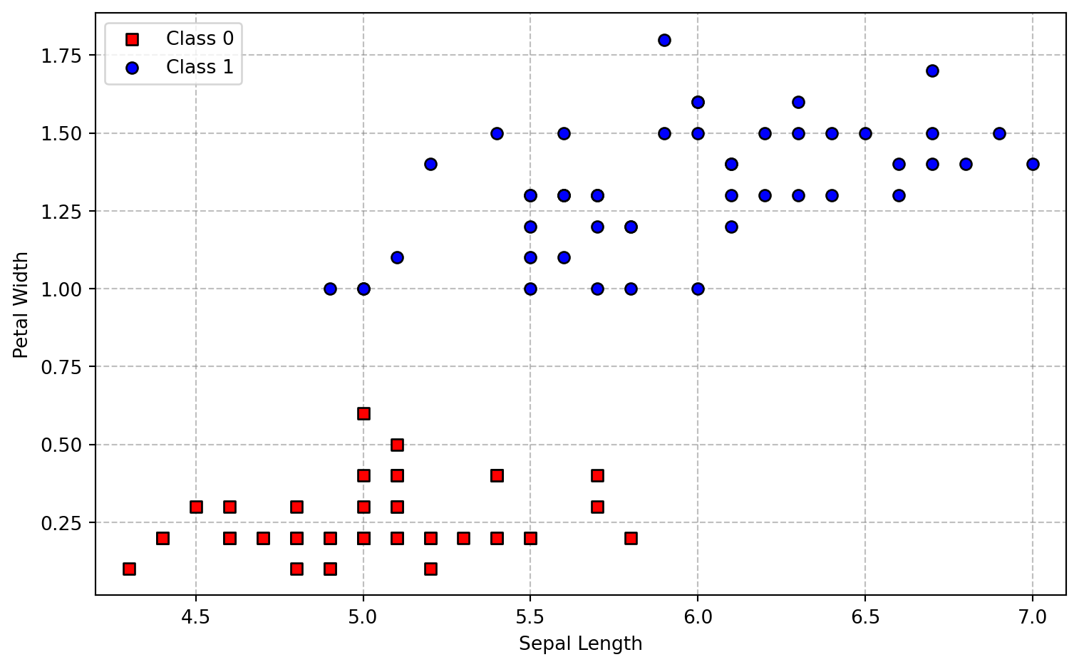
Come abbiamo già fatto con Adaline, testiamo il classificatore binario Logistic Regression con il
dataset Iris,
riutilizzando i metodi get_iris_data, plot_dataset_2D e plot_decision_regions:
import numpy as np
import matplotlib.pyplot as plt
import matplotlib.colors

X, y = get_iris_data()
plot_dataset_2D(X, y, x_label="Sepal Length", y_label="Petal Width")
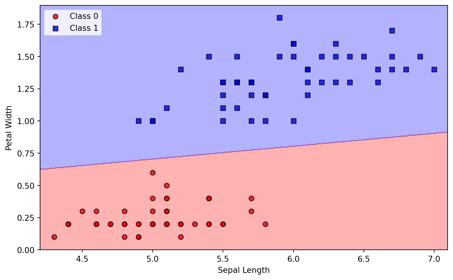
Utilizziamo l’intero dataset per eseguire il training del modello, e per mostrare a video le regioni decisionali, ed il relativo confine decisionale:
from matplotlib.colors import ListedColormap

# fit the Logistic Regression model and plot the decision regions
log_reg = LogisticRegressionGD(eta=0.5, epochs=200, random_state=2)
log_reg.fit(X, y)
plot_decision_regions(X, y, classifier=log_reg, resolution=0.005,
                      x_label="Sepal Length", y_label="Petal Width")
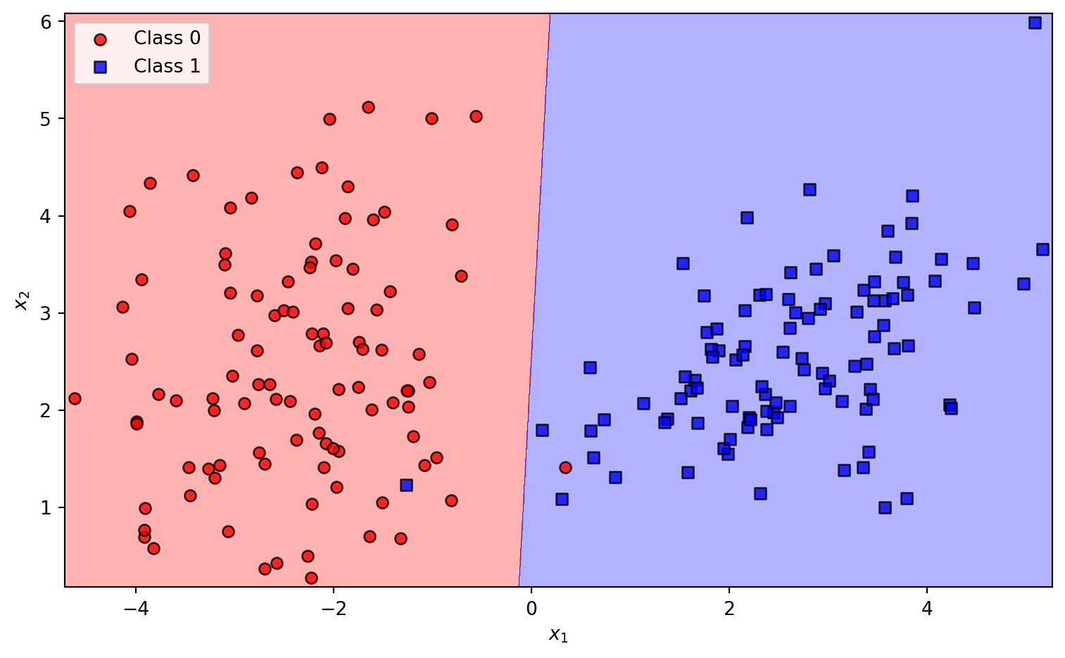
Un Dataset Sintetico
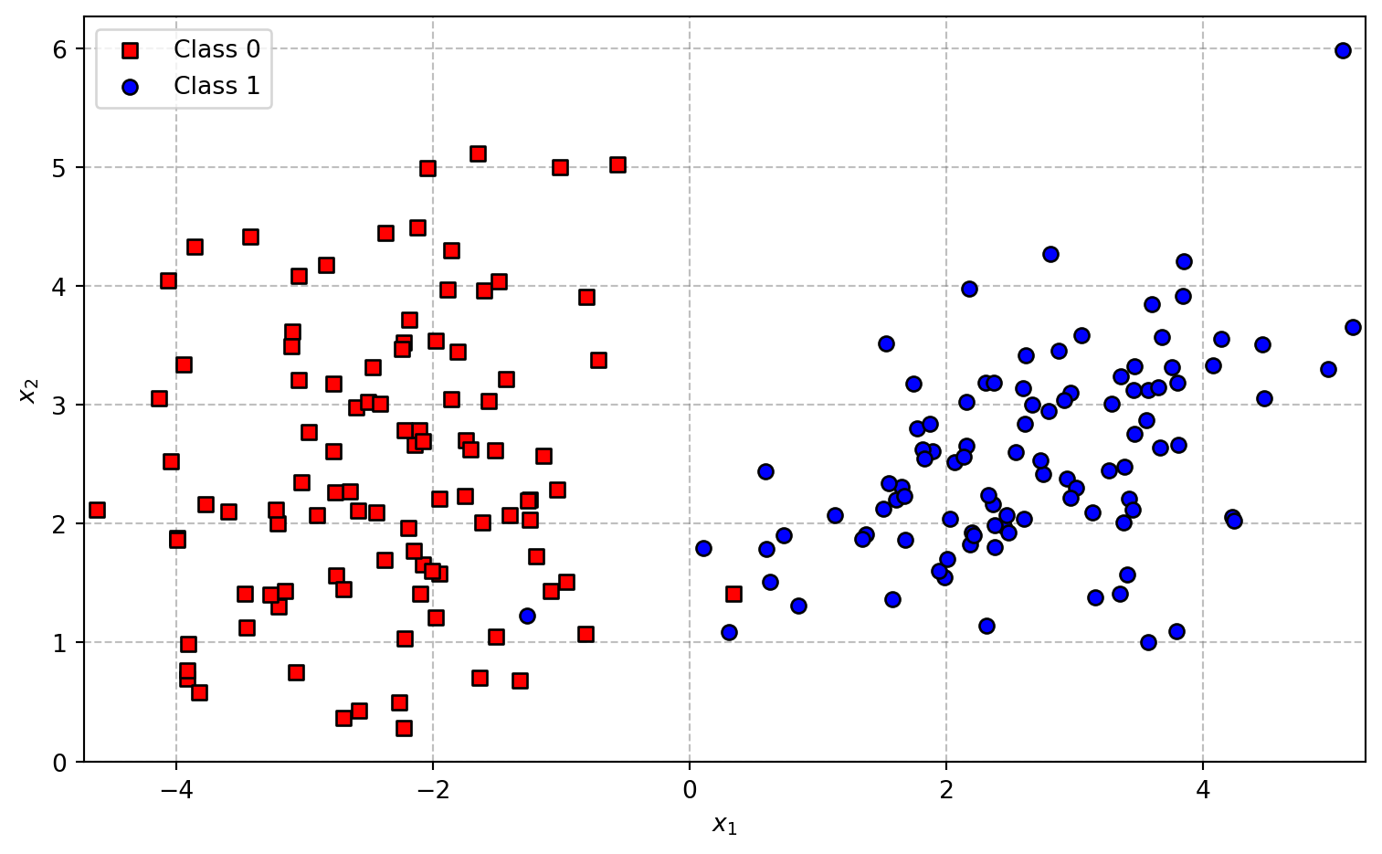
from sklearn.datasets import make_classification

# get data
X, y = make_classification(
    n_samples=200,
    n_features=2,
    n_redundant=0,
    n_informative=2,
    n_clusters_per_class=1,
    class_sep=2.5,
    random_state=42
)

plot_dataset_2D(X, y)
# fit the Logistic Regression model and plot the decision regions
log_reg = LogisticRegressionGD(eta=0.5, epochs=200, random_state=2)
log_reg.fit(X, y)
plot_decision_regions(X, y, classifier=log_reg, resolution=0.005)
Il Confine Decisionale
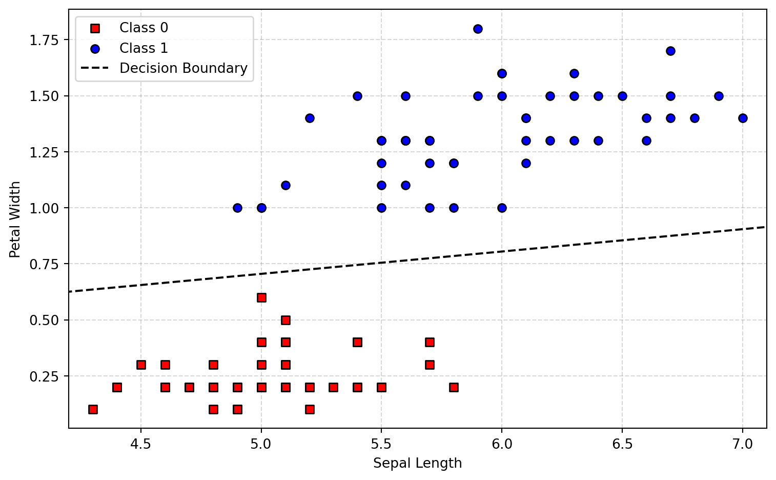
Nel contesto della classificazione binaria, il confine decisionale della Regressione Logistica è l’insieme di tutti i punti dello spazio delle feature per i quali il modello assegna la stessa probabilità alle due classi. Formalmente, esso è definito dall’equazione:
$$ \begin{align} \sigma\left(z\right) & = p = 0.5 \label{dec_bound_1}\tag{1}\\[6pt] \end{align} $$dove la funzione Sigmoide è definita come:
$$ \begin{align} \sigma\left(z\right) & = \frac{1}{1 + e^{(-z)}} = \frac{1}{1 + e^{(-\textbf{w}\textbf{x} + b)}}\label{sigmoid}\tag{2}\\[6pt] \end{align} $$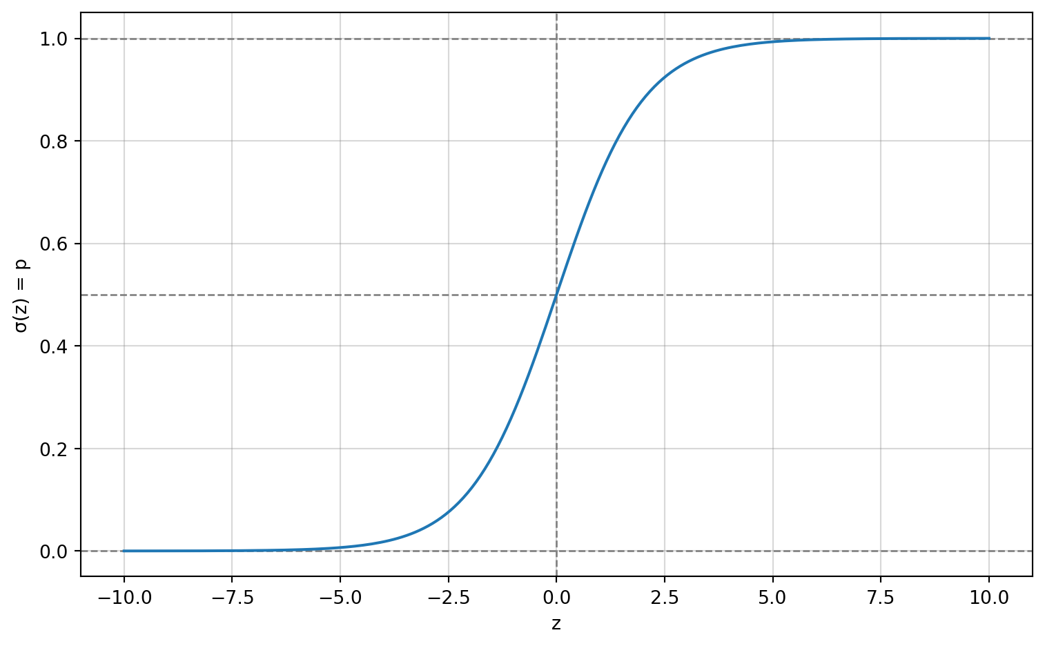
Il confine decisionale rappresenta quindi l’insieme delle osservazioni di input per le quali il modello è indifferente tra le due classi, ossia quando la probabilità predetta per la classe positiva è esattamente pari a $0.5$. Poiché la funzione Sigmoide restituisce il valore $0.5$ quando il suo argomento (logit) $z$ è uguale a zero, la condizione precedente equivale a imporre:
$$ \begin{align} z & = w_1x_1 + \dots + w_nx_n + b = 0\label{logit}\tag{3}\\[6pt] \end{align} $$L’equazione $\eqref{logit}$ è un’equazione lineare nello spazio delle feature, e rappresenta un iperpiano in uno spazio di dimensione $n + 1$, dove $n$ è il numero di feature. Questa equazione descrive una superficie piana e rettilinea: per questo motivo il confine decisionale della Regressione Logistica è sempre lineare.
Dal punto di vista visivo, la funzione Sigmoide non altera la forma del confine decisionale, poiché non viene utilizzata per calcolare direttamente la funzione di ipotesi. Il suo ruolo è esclusivamente quello di trasformare il valore del logit — ossia l’output della funzione di ipotesi, o weighted sum — in una probabilità compresa tra $0$ e $1$. In questo modo, gli errori lineari (valori reali non limitati, “unbounded”) vengono convertiti in errori probabilistici, rendendo possibile sia un’interpretazione probabilistica del modello, sia l’addestramento tramite la funzione di costo Cross-Entropy.
Poiché la Sigmoide vale $0.5$ solo quando il suo argomento è $0$, il confine decisionale della Regressione Logistica coincide con l’insieme dei punti che soddisfano l’equazione $\textbf{w}\textbf{x} + b = 0$. A livello geometrico, la Sigmoide “colora” lo spazio con probabilità, ma il confine decisionale è la linea (o iperpiano) che passa esattamente nel punto in cui il colore cambia da “classe 0 più probabile” a “classe 1 più probabile”.
Ad esempio, nel caso di un vettore di feature bidimensionale $\textbf{x} = \left({x}_1, x_2\right)$ e di un termine di bias $B$, l’equazione del confine decisionale diventa:
$$ \begin{align} z & = w_1x_1 + w_2x_2 + B = 0 \label{dec_bound_2}\tag{4}\\[6pt] \end{align} $$Risolvendo l’equazione rispetto a $x_2$, otteniamo:
$$ \begin{align} x_2 & = -\frac{w_1x_1 + B}{w_2} \label{dec_bound_3}\tag{5}\\[6pt] & = -\frac{w_1}{w_2}x_1 -\frac{B}{w_2} \label{dec_bound_4}\tag{6}\\[6pt] \end{align} $$L’equazione $\eqref{dec_bound_4}$ può quindi essere interpretata come l’equazione della retta del confine decisionale nella sua forma esplicita:
$$ \begin{align} y & = mx + b \label{line-eq-point-slope}\tag{7}\\[6pt] \end{align} $$dove il coefficiente angolare $m$ e il termine intercetta $b$ sono definiti come:
$$ \begin{align} m & = -\frac{w_1}{w_2}\label{slope}\tag{8}\\[6pt] b & = -\frac{B}{w_2}\label{bias}\tag{9}\\[6pt] \end{align} $$Avendo i valori di $m$ e $b$, possiamo utilizzare l’equazione $\eqref{line-eq-point-slope}$ per tracciare la retta del confine decisionale.
Pertanto, ogni osservazione situata da un lato del perimetro apparterrà alla classe “$1$”,
mentre ogni osservazione situata sul lato opposto apparterrà alla classe “$0$”.
Vediamo un’esempio, nel quale il metodo plot_dataset_2D prende i parametri weights e bias del classificatore di input,
e li usa per disegnare tale retta:
from sklearn import datasets

def get_iris_data():
    """This data sets consists of 3 different types of irises: 'Setosa', 'Versicolour' and 'Virginica'.
    There are 150 examples, 50 examples for each class.
    The features are: 'sepal length', 'sepal width', 'petal length' and 'petal width'."""
    iris = datasets.load_iris()
    X = iris.data[:, [0, 3]]  # just consider "sepal length" and "petal width"
    y = iris.target
    X = X[0:100]              # class 0 and class 1
    y = y[0:100]              # class 0 and class 1
    return X, y

def plot_dataset_2D(X, y, classifier: LogisticRegressionGD, plot_decision_boundary=True,
                    x_label="$x_1$", y_label="$x_2$"):
    """Draw a scatter-plot of the input Iris data."""
    markers = ("s", "o")
    colors = ("red", "blue")
    plt.figure(figsize=(8, 5))

    # plot class samples
    for idx, cl in enumerate(np.unique(y)):
        plt.scatter(x=X[y == cl, 0], y=X[y == cl, 1],
                    marker=markers[idx], label=f'Class {cl}',
                    c=colors[idx], edgecolor="black", zorder=2)

    # plot decision boundary
    if plot_decision_boundary:
        xl = np.linspace(X[:, 0].min() - 1, X[:, 0].max() + 1, num=100)
        w = classifier.weights  # get classifier's weights
        B = classifier.bias     # and bias
        m = -w[0]/w[1]          # compute the m and b parameters
        b = -B/w[1]             # of the decision boundary line
        yl = m*xl + b           # then use the line equation to compute the line's y coordinates
        plt.plot(xl, yl, c="black", linestyle="--", alpha=1.0, zorder=2, label="Decision Boundary")

    plt.xlabel(x_label)
    plt.ylabel(y_label)
    plt.legend()
    plt.xlim(X[:, 0].min() - 0.1, X[:, 0].max() + 0.1)
    plt.grid(color='gray', alpha=0.3, linestyle='--')
    plt.tight_layout()
    plt.show()

# get data
X, y = get_iris_data()

# instance and train the model
log_reg = LogisticRegressionGD(eta=1, epochs=200, random_state=2)
log_reg.fit(X, y)

# plot the dataset, and the model's decision boundary
plot_dataset_2D(X=X, y=y, classifier=log_reg,
                x_label="Sepal Length", y_label="Petal Width")